Understanding and optimizing gas compressor stations
May 10, 2021
Many gas compressor stations use multiple gas turbine-driven centrifugal compressors. Experts from Solar Turbines describe a variety of optimization methods and illustrate the capability of methods that combine optimization of turbomachinery and pipeline hydraulics.
Fuel optimization for compression applications has to consider the application characteristics as well as the characteristics of the drivers and compressors involved.
The present study attempts to provide a generalized view that involves consideration of the equipment in a station. I can also can include the behavior of the entire compression system, using a pipeline with multiple compressor station as an example. Different compressor control modes are considered and very simple, as well as more complicated concepts are introduced.
This paper assumes two shaft gas turbines as drivers and centrifugal compressors as the driven equipment. It considers the impact of the change in gas turbine efficiency with load and speed.
The available gas turbine power depends on ambient conditions as well as the power turbine speed. The gas turbine efficiency additionally ids a function of the gas turbine load, with the best heat rate at full load.
The driven compressor for the applications in question is typically a centrifugal compressor, which is either directly or via a fixed ratio gearbox coupled with the power turbine. varying its speed is therefore the most effective and efficient way of controlling the compressor operation.
It should be noted that ’control by varying the speed’ does not mean ‘controlling the speed’. The control mode typically applies to a process parameter, for example suction pressure, discharge pressure or flow. Any deviation from the controlled parameter will lead to an adjustment of the engine power output, which will result in a change in compressor speed.
Different ways of load sharing are possible if multiple units operate in a station. Two frequently used methods involve to either keep all engines at the same relative load, or to keep all driven compressors at the same distance from their surge line, thus at the same turndown. Turndown is defined as the distance of the compressor operating point from the surge line for constant head.
The operating point of the driven compressor is determined by the system in which it works. The system, for example a pipeline upstream and downstream of a compressor station, imposes the suction and discharge pressure on the compressor. And the compressor reacts to it, based on the power available, with a certain flow.
The flow in turn may alter the suction and discharge pressure that the system imposes on the compressor. Some systems have a strong impact of the flow on the pressure levels, as the pressure losses of pipelines are directly related to the flow through these pipelines. Other systems may show very little change in suction and discharge pressure with flow.
Minimizing fuel consumption is not the only optimization goal used. Other characteristics that play a role include maximizing availability, possibly also for short-term events, leading to partly loaded units in anticipation of a rapid increase in load (in the world of power generation, this would be called a spinning reserve). Minimizing the number of starts, or minimizing running hours could be other requirements.
When a compressor station, or a number of related compressor stations in a pipeline are planned, certain considerations have to be made. The first consideration involves the capability to cope with changes in flow capacity on all time scales, that is hourly, daily, seasonally.
Contractual requirements and obligations, such as pressures and volumes at transfer points, have to be considered. The second consideration deals with the fact that the nominal capacity of a pipeline may grow when additional customers demand a higher supply of natural gas. In fact, many new pipelines start out with 50 percent and less capacity and grow to full capacity over several years, or are sized for easy expansion.
Other applications, for example in upstream application, will also experience changes in suction pressure and flow due to declining fields.
The total cost of ownership reflects the cost to install, operate and decommission the stations. While the first two considerations reflect the capability to generate revenue, the latter focuses on the necessary costs. These costs (ci) may appear at any point in time during installation, operation and decommissioning of the station. Revenue reduction resulting from equipment downtime is an important element of the total cost of ownership.
Studies at the start of the planning process will typically assess the station size. For pipelines, the starting point is the distance the pipeline has to cover and the amount of gas that needs to be transported. Optimization studies then will assess the impact of pipe diameter, operating pressure, number of compressor stations.
Tradeoffs include the cost for the pipe, the cost for the compression equipment and the operation cost for the different choices. Larger pipes reduce the amount of compression power to be installed, but increase the cost for the pipe.
Having stations closer together reduces the amount of power to be installed, and reduces the fuel cost but increases maintenance requirements. Figure 1 shows the result of such an evaluation, with the recommendation for a 28-inch pipe, and a compressor station pressure ratio of about 1.3 to 1.4.
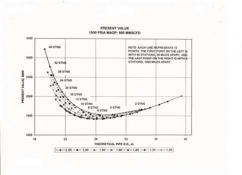 Figure 1: Pipeline optimization results
Changing operating conditions
While some compressor stations are more or less operated at constant load, many installations see widely fluctuating operating conditions. These fluctuations are, in concept, foreseeable in the planning stage.
Give the load dependency of the driver efficiency, a station that runs under a wide range of loads will often operate in part load, thus incurring higher fuel consumption. That is unless one has multiple units, with the option to shut down units, rather than operating in part load.
We will first discuss the desirable number of compressors in station in relation to the range of load fluctuations. We then will discuss the impact of changing ambient temperature. Since the engine output changes with the inlet temperature, even at constant station flow demand (that is, with the compressors consuming constant power), the engine load (relative to their maximum available power) can fluctuate with changing ambient temperatures.
Comparing the impact of variability
Case A (Figure 2), for a station with large swings in load, exhibits a clear advantage of multi-unit stations. As the smaller units are operated closer to full load for most of the time, the resulting fuel usage is lower than for single-unit stations. This holds true for both slopes in part-load efficiency, and even if the smaller units achieve a lower base efficiency than the larger units. For virtually all cases, a station with three or four units minimizes the fuel usage. Additional units yield no additional benefits.
Case B, typical for large pipelines with few take-offs, gives a different picture. Comparing Figure 3 shows that the conclusion regarding the optimum number of stations depends highly on the baseline efficiency of the packages involved. If the smaller units have the same design efficiency as the larger units, then a three-unit station is advantageous. If we assume lower efficiencies for the smaller units than for the larger units, a one or two unit station uses less fuel.
Both Figures 6 & 7 distinguish between gas turbines with steeper (Series 2) and less steep reductions (Series 1) in part load efficiency. Both pictures on the left assume an efficiency advantage for larger units. The minimum in fuel usage also implies a minimum in CO2 production.
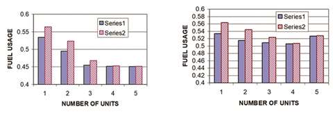 Figure 2: Case A shows a clear advantage of multi-unit stations
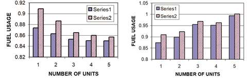 Figure 3: Case B concludes that the optimum number of stations depends highly on the baseline efficiency of the packages involved
It again needs to be emphasized that a station outage may cause significantly higher cost, due to lost revenue rather than the fuel cost for an entire year. A standby unit significantly reduces the exposure. If the station uses multiple units, then the unavailability of one of these units has a smaller impact on the amount of gas that can be produced. Admittedly, the chances that one out of four units fails are higher than the chances that one out of two units fail.
 Figure 4: Two units vs three units, capability to shut a unit down
Besides fluctuations in the required compressor power we also find situations where the ambient temperatures show large swings, especially between summer and winter conditions.
The situation during low ambient temperatures may allow to shut a unit down entirely, depending on the number of units in a station. The compressors in operation will see a larger flow (Figure 4) if the station flow is to be maintained.
Figure 4 illustrates the advantage of smaller units (three units in a station) over larger units (two units in a station). The station with three units can accommodate the shut down of a unit. Yet the compressor that remains in operation will not be able to handle the increased flow for a station with two units. Shutdown of units, instead of running units in part load, has a positive impact on fuel consumption (Figure 5) and maintenance cost (a unit that is shutdown does not accrue fired hours, a unit operating in part load does).
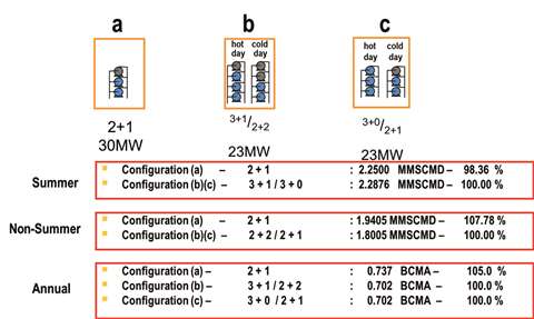 Figure 5: Shutdown of units, instead of running units in part load, has a positive impact on fuel consumption
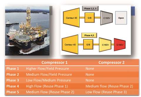
In cases where the operating conditions change significantly over time, which is a situation frequently encountered in installations near oil or gas fields, concepts that take advantage of package flexibility may be considered.
The example (Figure 6) shows a situation at a declining gas field, where gas flow and suction pressure dropped over time.
The addition of another compressor to the train to accommodate the declining suction pressure, and the resulting increase in pressure ratio had been planned, so the skid was prepared to accept an additional compressor body. Together with targeted restages, that allowed to re-use existing aerodynamic hardware, the wide range of operating conditions was covered (Figure 6).
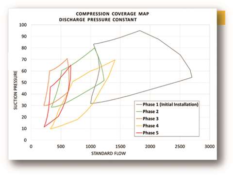 Figure 6: Declining gas field, where gas flow and suction pressure dropped over time (above and below)
Basic operations optimization
Simple yet very effective methods include the concept to load all involved units evenly, and to run the least amount of units necessary.
The downside of this approach is, that if done consistently, the number of starts and stops for the units may increase. Loading units evenly can either be accomplished by running all compressors at the same distance from their respective surge line, or by running all gas turbines at the same load setting, for example by equalizing their gas producer speed relative to the speed at full.
Additional considerations are required if the units involved are different in size and operating characteristics. Many compressor stations combine units of different size and vintage. The newer units may be less expensive to operate, may have a higher fuel efficiency and may be bigger (in terms of power output) compared to the older units. One of the key tasks may be to re-stage the compressors of the older units in order to be able to contribute at a reasonable cost to the station operation. For the purpose of this study, we assume that this has happened.
More involved methods would include simulations of entire systems. For example, of a pipeline with multiple compressor stations and multiple compressor units per station) using numerical simulations.
Here is an example of a simple yet very effective scheme. Let us assume we have a compressor station with one large unit (KC) and three smaller units (TC) all operating in parallel. For simplicity, the smaller unit produces half the power of the larger unit:
And the compressors are aerodynamic scales, thus maintaining aerodynamic similarity. The parallel operation forces all units to operate at the same suction and discharge pressure. Based on the above, the total available station power P = 5 PTC.
We can now define different load Steps:
Step 1 P=PTC;
Step 2 P=PKC or P=2 PTC;
Step 3 P=PKC + PTC or P=3 PTC;
Step 4 P=PKC + 2PTC, and;
Step 5 P=PKC + 3PTC.
For all power demands that are higher than Step n, but lower than Step n+1, the running units are equally loaded.
Further considerations have to be made to decide which options should be pursued for Steps 2 & 3. One consideration could be maintenance cost. It could well be that the larger unit accrues lower maintenance cost per fired hour than two of the smaller units. Similarly, if the larger unit is more efficient than the small units, one would opt for starting the larger unit in Steps 2 & 3.
Another option would be to analyze typical load cycle for the station. If the load typically rises beyond Step 3 relatively fast, it might be advantageous to start the large unit in Step 2. If the load often just stays between Steps 1, 2, & 3 (as is the case for stations that have seasonally lower loads), then these Steps may be better covered by the smaller units.
The simulations in this section assume compressor operating points at constant head. The flow therefore changes with the amount of power supplied to the compressor. The change in compressor efficiency and operating speed are accounted for in the simulation. Also, the gas turbine power output and heat rate are adjusted for power turbine speed and load. The available power is based on realistic site conditions.
The station in question is analyzed based on one or two units of 15MW (20,000hp) and 22.5MW (30,000hp) compressor sets (Figure 7).
The 22.5MW (30,0000hp) sets are assumed to have a higher overall efficiency than the 15MW (20,000hp) sets. Individual gas turbines are used for very low flows. With increasing flow, the combinations used go from two times 15MW (20,000hp) units to one 15MW (20,000hp) and one 22.5MW (30,000hp) unit, and finally to two times 22.5MW (30,000hp) units. There is overlap between the different configurations. The addition of a unit increases the fuel flow initially, as two units now operate in part load instead of one unit at full load.
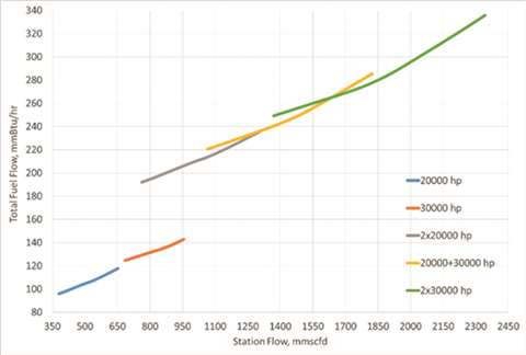 Figure 7: Various Equipment combinations in operation, fuel flow versus compressed gas flow
Similarly, for all higher flow cases it is advantageous to run the unit combinations up to their full load capability before turning on additional or bigger units.
Figure 8 shows the results of the simulations for different control methods at a compressor station with two compressor sets of different size (Unit 1 with 1.5 times the power of Unit 2). Compared are the cases where the units are equally loaded (with either the small or the big unit leading) or where they are controlled for equal turndown.
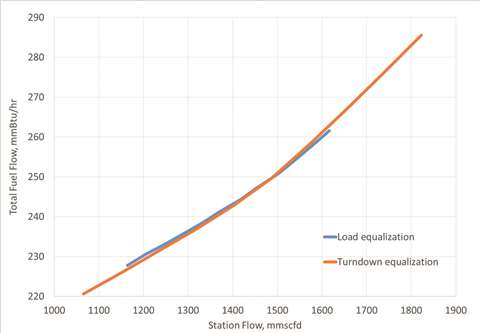 Figure 8: Load equalization. Equal load, with the 15MW or the 22.5MW engine leading versus equal turndown for the compressor
Equal load is usually accomplished by controlling the gas producer speed of the gas turbine. The fuel consumption for a certain station flow demand is about the same for either control method. There is a significant advantage for the equal turndown method at low and high flows, where the equal load method is limited either by surge line on one unit or by maximum speed on another.
Turndown equalization has a wider allowable flow range since it is more tied to compressor maps, and initially the compressor selection had been done based on turndown evaluation not engine load. It is probable to find compressor selections, which will provide the same operating range, if we are at station design and if there is a particular request to find optimized solution based on sharing the load equally. However, it might be easier just to use turndown equalization.
Optimizations that involve multiple but connected compressor stations require the modelling of the connecting pipes, meaning that pipeline hydraulics have to be considered. This will lead to a number of constraints for the individual compressor station, that are not obvious on the station level. A key feature is, that for a pipeline, pipeline flow and station pressures are not independent. That means if the flow through the pipeline is increased, the pressure ratio for the compressor station has to increase.
Variable speed centrifugal compressors are uniquely suitable for this type of operating characteristic. This is because all steady state points can be placed near the bets efficiency are of the compressor, while the wide range allows for suitable deviations imposed by non-steady state operation. Even with massive load changes (for example by bringing the driver form 50% to 100% load within less than a minute), the compressor will not operate at constant head and varying flow for more than a few seconds.
Figure 9 shows the layout of such a pipeline of a given length (Ltot), five compressor stations (station 1 through to 5) at roughly equal distance, and a side stream entering the main pipe just upstream of station three.
The simulation takes into account the fuel consumption of each of the five stations, as well as the line pack (ie the gas stored in the pipeline system itself). The pipeline geometry (diameter, roughness), maximum allowable operating pressure (MAOP), site elevations and local ambient temperatures are known.
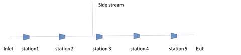 Figure 9: Pipeline schematic that takes into account the fuel consumption of each of the five stations as well as the line pack
The compressor stations use a variety of different centrifugal compressors, all of them driven by two shaft gas turbines. Recycle of individual units, as well as shut down of individual units is possible and has to be considered as part of the simulation. Also the entire station can be bypassed. A summary of the installed units is in Table 1.
The actual operating conditions for all units were used as a starting point in the study. In this situation, all but two units in station 5 were running, and all of them at relatively low load (Table 2). The optimized scenario consumed 74% of the fuel compared to the original situation.
The two major contributing factors are the smaller number of units running at higher load, and the generally lower gas velocity in the pipe (Figure 10), which significantly reduced the pressure losses. This was accomplished by running station two with more units at a higher load. The higher load on station 2 was achieved by running at higher head despite being in recycling.
Table 1: Installed power
| Station | Number of units | Power class of Units (MW) | Total Installed Power (MW) |
| 1 | 0 | 0 | 0 |
| 2 | 2 | 14.5 | 2.9 |
| 3 | 2 | 15.3 | 30.9 |
| 4 | 2 | 15.3 | 30.9 |
| 5 | 5 |
3 ea 6 1 ea 7.8 1 ea 11.2 |
37 |
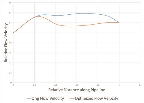 Figure 10: Optimizing the fuel consumption. Shifting load between stations allows to lower the flow velocities, and the pressure drop in the pipeline
Apart from the optimization of the pipeline hydraulics, it can also be seen that the recipe given in the previous section seems to be approximately replicated by the numerical optimization.
Table 2: Station load
|
Station |
Number of units running |
Average load of running units |
Number of units running (optimized) |
Load of running units (optimized) |
| 1 | 0 | N/A | 0 | N/A |
| 2 | 2 | 56% | 2 | 70% |
| 3 | 2 | 57% | 1 | 94% |
| 4 | 2 | 63% | 1 | 83% |
| 5 | 3 | 96.6% | 1 | 97% |
Understanding the behavior of turbomachinery equipment and the overall system allows appropriate methods for fuel and operational optimization on the station level and for entire pipelines. Optimization can and should happen both during the planning of the system, as well as during the operation of a system.
Key influence factors in the planning phase include the number of stations and units, based on assessments on the variability of the operating conditions. Variability will occur on various timescales.
During the operation relatively simple rules can be derived based on the conceptual understanding, or from evaluation of more complex studies. The concepts described work even if units are not identical, and can entirely be based on measurable parameters.
The challenge is to control the units so that certain operational parameters, for example fuel consumption, are optimized. The control system has to rely on measurable parameters, even if parameters that are not directly measured (such as the gas composition for the compressor) change during operation.
Methods to control all compressors for the same turndown provide good results regarding efficiency and operating range, compared to controlling all gas turbines for the same load. Modelling the entire pipeline allows further optimization, which cannot be achieved if the optimization is performed at the station level only.
US-based experts from Solar Turbines
 Rainer Kurz. Manager for systems analysis & field testing in San Diego
 Matt Lubomirsky. Consulting engineer of systems analysis in San Diego
 Avneet Singh. Manager for gas compressor performance & applications in San Diego
 Roman Zamotorin. System analysis engineer in Houston
MAGAZINE
NEWSLETTER


CONNECT WITH THE TEAM